This years ICLR was was special for me (and for many others as well) as it was the first virtual conference I have ever attended to (and will given the current situation with COVID-19 surely not be the last). At the virtual ICLR, posters were replaced with short prerecorded videos of 5 minutes where the authors briefly present their work. These videos can be accessed at any time independent of the “poster session” in which was possible to talk to one or more authors of the paper. One benefit of the conference being completely virtual is definitely that it allows to spread out looking at the “posters” over a longer time (if willing to sacrifice the possibility to talk with the author in a virtual poster session).

Overall, I found this format very appealing, as it allows to get a quick perspective into the work and also allows to look at many works without getting overwhelmed as the presentations are usually kept at a high level. For more detailed information it is always possible to pull up the paper.

A few weeks after the virtual conference is over I finally managed to summarize some of the papers and posters I looked at, and thought I might as well share it with the people who could be interested. You can find a subset of the papers I selected for reading accompanied with a sometimes more, sometimes less detailed summary below. I must say that I am still not completely finished with all the papers I marked and thus might update this page at a later time.

Table of Contents

• Table of Contents
• Anomaly Detection
  • Deep Semi-Supervised Anomaly Detection
  • Input Complexity and Out-of-distribution Detection with Likelihood-based Generative Models
• Generative Models
  • Understanding the Limitations of Conditional Generative Models
  • Your classifier is secretly an energy based model and you should treat it like one
• Gradient Estimation
  • Estimating Gradients for Discrete Random Variables by Sampling without Replacement
  • SUMO: Unbiased Estimation of Log Marginal Probability for Latent Variable Models
• Pooling and Set Functions
  • FSPool: Learning Set Representations with Featurewise Sort Pooling
  • On Universal Equivariant Set Networks
  • StructPool: Structured Graph Pooling via Conditional Random Fields
• Representation Learning
  • Disentanglement by Nonlinear ICA with General Incompressible-flow Networks (GIN)
  • InfoGraph: Unsupervised and Semi-supervised Graph-Level Representation Learning via Mutual Information Maximization
  • Mutual Information Gradient Estimation for Representation Learning
  • On Mutual Information Maximization for Representation Learning
• Seq2Seq models
  • Are Transformers universal approximators of sequence-to-sequence functions?
  • Mogrifier LSTM
  • Reformer: The Efficient Transformer
• Understanding Deep Learning
  • Four Things Everyone Should Know to Improve Batch Normalization
  • On the Variance of the Adaptive Learning Rate and Beyond
  • The Implicit Bias of Depth: How Incremental Learning Drives Generalization
  • Towards neural networks that provably know when they don’t know
  • Truth or backpropaganda? An empirical investigation of deep learning theory
  • What graph neural networks cannot learn: depth vs width
  • Why Gradient Clipping Accelerates Training: A Theoretical Justification for Adaptivity
• Other - Normalizing Flows, Robustness, Meta-Learning, Probabilistic Modelling
  • Invertible Models and Normalizing Flows
  • Learning to Balance: Bayesian Meta-Learning for Imbalanced and Out-of-distribution Tasks
  • Meta Dropout: Learning to Perturb Latent Features for Generalization
  • On Robustness of Neural Ordinary Differential Equations
  • Why Not to Use Zero Imputation? Correcting Sparsity Bias in Training Neural Networks

Anomaly Detection

Deep Semi-Supervised Anomaly Detection

Anomaly detection in the Semi-supervised setting: Additional labels samples to leverage expert knowledge

Goal: Improve decision boundary using the labeled data.

A supervised classifier usually performs bad on unseen samples. Unsupervised approaches cannot use the labels examples to improve.

Suggest the Deep SAD method with is an extension of the Deep SVDD method. The SAD method is unsupervised and tries to map examples (non-anomalies) into a as compact as possible hypersphere.

(I wonder how this is different to maximum likelihood training of a simple generative models such as a flow? In the end we simply penalize the distance from the mode. Of course this approach does not penalize contraction / stretching of the space such that it can map all examples to a very small volume).

The SVDD approach tries to minimize the following objective:

and the authors of this paper suggest including an additional term which penalizes anomalous samples from being close to the center of the sphere. The objective then becomes:

where $y_j=1$ for normal samples and $y_j=-1$ for anomalies.

Makes perfect sense. Additionally, the authors benchmark their method and present an information-theoretic framework for deep anomaly detection in their paper.

Input Complexity and Out-of-distribution Detection with Likelihood-based Generative Models

Obvious strategy of generative models for detecting OOD samples (train model on data, label low likelihood samples as OOD) does not work. Often the out of distribution samples actually have significantly higher likelihood than the training distribution.

Intuition of paper: The input complexity of the dataset images influences the likelihood.

Analyse normalized size of image after being compressed with lossless compression which serves as a proxy for the Kolmogorov complexity. Complexity of image seems to correlate with the likelihood (more complex, less likely). Most variance is explained by this.

Suggest to correct the likelihood by subtracting the complexity estimate of the image, and show that this can be interpreted as a likelihood ratio test statistic giving links to Bayesian model comparison, minimum description length and Occams razor.

Results indicate higher performance compared to many out of distribution detection methods. The only method based on generative modelling which out performs the approach is WAIC which relies on ensembles of generative models and thus is sufficiently more costly to optimize.

Input complexity is the main culprit for out of distribution detection and proxies of input complexity can be used to to design corrected scores.

Generative Models

Understanding the Limitations of Conditional Generative Models

Main problem of conditional generative models: Not robust, do not recognise out of distribution samples.

Ideally, in a good generative model undetected (high density) adversarial attacks should have a low volume. Problem: Even if adversarial attacks are close to this low volume set the close area itself would again be large due to the curse of dimensionality. The theory of the paper suggests that one can always construct such a adversarial attack such that it would not be detected (?, have to check on this in the paper).

Results: MNIST model is robust, CIFAR model to detect. –> Interpolated examples (in data space) on CIFAR have higher likelihood than the samples themselves Explanation: Classification and Generation are very different things. Classification only cares for very few aspects of the data, while generation tries to model every single aspect of the data.

The authors suggest that the class-unrelated entropy (background, nascence variables) in CIFAR is the reason for these models failing. Demonstrate this with new dataset where MNIST digits are on CIFAR background and thus increasing the class-unrelated entropy. Then MNIST also fails similarly to CIFAR in the previous example.

Authors argue that much of the problem comes from the standard likelihood objective which tries to model everything, while for classification one only cares about selected bits of the data.

Your classifier is secretly an energy based model and you should treat it like one

Criticism: Progress in generative models driven by Likelihood and sample quality. Not by downstream tasks such as:

• Out of Distribution detection
• Robust classifications
• semi-supervised learning In practice, the generative model based solutions on these tasks usually lag behind compared to engineered solutions. Why?
• Not flexible enough?
• Architecture only good for generation not classification etc.
• Additional modelling constraints are making models worse for discrimination (such as invertibility for flows)

Alternative: Use energy based models!

• Very flexible! We only need a energy function
• But we cannot easily compute the normalizing constant which leads to some problems with regard to sampling and training

How to train? While log likelihood does not have a nice form, the gradient of log p can be written quite simply:

where the last term is evaluated on the data and the first uses samples from the model (which is also tricky, usually done using MCMC).

Contribution:
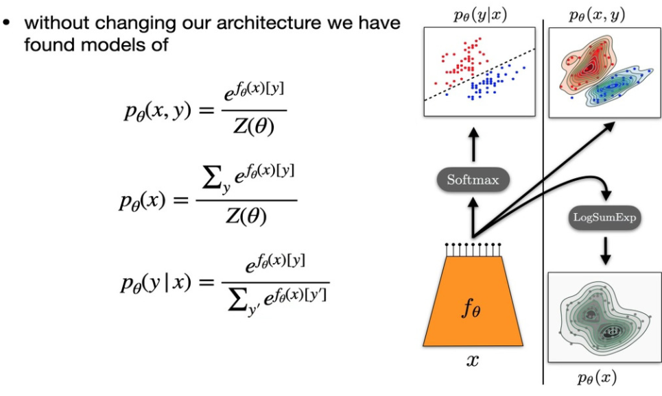
Take classifier models and instead of using softmax define a energy based model using the inputs before the softmax. Where the energy is the negative output of the class indexed preactivations: $E_{\theta}(x, y) = -f_{\theta}(x)[y]$ This EBM can be trained and later used to predict the class using basic rules of probability, which simply results in a softmax. Further we can sum $y$ out to which also results in a EBM of the form: $E_{\theta}(x) = - LogSumExp_y(f(x)[y])$, which is a purely generative model.

What to do with this insight? - Experiments
Train factorized distribution to ensure unbiased training of classifier: $p(x) + p(y|z)$ as it does not require sampling from the joint distribution which could be biased. (This is actually reflected in the results, which show poor performance when the distribution is factored). Nevertheless, this hybrid model is the only one which yields comparable classification performance to STOA. Further, JEM improves calibration of the models significantly compared to baseline approaches. Also the JEM model is better at recognizing out of distribution samples and adversarial examples. This is done using a trick where they seed the MCMC chain at the position of the adversarial sample and execute a few MCMC steps with respect to the learned data distribution, further improving adversarial robustness significantly.

Nevertheless, training is still very unstable due to MCMC sampling. Learning is also hard to diagnose as there is no clear loss definition.

Gradient Estimation

Estimating Gradients for Discrete Random Variables by Sampling without Replacement

Discrete variables do not allow the computation of a gradient which is needed for gradient based optimization. This problem is usually mitigated by one of two approaches:

• Relaxation of the discrete distribution to a continuous distribution (+ evtl. sampling) such as Gumbel-Softmax or Concrete methods. These unfortunately usually have a high bias.
• Sampling and deriving stochastic gradients usually based on REINFORCE. REINFORCE gradients usually have high variance.

Authors say that REINFORCE is basically a “trick” for pulling the gradient operation inside the expectation:

Further, one can use the average of the other samples in order to reduce the variance of the estimate (REINFORCE with baseline, Mnih & Rezende 2016):

In contrast to previous work the authors suggest to sample without replacement, as duplicate samples are uninformative in a deterministic setting. This leads to a sequence of ordered samples drawn from the distribution such that

In their paper, they derive a generic estimator for $E[f(x)]$ by Rao-Blackwellizing the crude single sample estimator (which is based on a single Monte Carlo sample). They call this estimator the unordered set estimator:

where $R(S^l, s) = \frac{p^{D \setminus { s } } (S^k \setminus { s } )}{p(S^k)}$ is the leave-one-out ratio and $S^k$ is an unordered sample without replacement. They then apply REINFORCE to the derived estimator for the computation of gradients which gives rise to the unordered set policy gradient estimator:

where the last step can be derived using the log derivative trick.

Further, the authors use an approach similar to Mnih & Rezende (2016) in order to reduce the variance by subtracting a baseline based on the other samples. This is not entirely trivial though, as the samples are not independent and thus a correction needs to be applied.

Experiments:

• Synthetic example: Shows lowest gradient variance compared to all other methods
• Policy for travelling salesman problem: Comparable to biased approaches and out-performs all unbiased approaches

The devised estimator is a low variance unbiased estimator which can be used as a replacement to Gumbel-Softmax.

SUMO: Unbiased Estimation of Log Marginal Probability for Latent Variable Models

Suggest a new gradient estimator for marginal probabilities.

Maximum likelihood estimation for Latent Variable Models (LVM) requires unbiased estimates of $\nabla_\theta \log p_\theta(x)$ which are not directly available. Instead research has focused on developing lower bounds for the log marginal probability $\log p_\theta(x)$ such as the ELBO or IWAE and to optimize the model parameters with respect to this lower bound.

The approach devised in this paper is composed of two components:

• Importance weighted bounds (IWAE): Here the idea is to use multiple samples, instead of a single sample as suggested with the ELBO. This results in an increasing tighter bound on the true marginal log-likelihood, such that

  \[\begin{gather} ELBO \leq E[IWAE_1(x)] \leq E[IWAE_2(x)] \leq \dots \leq \log p_\theta(x) \\\\ \log p_\theta(x) = \lim_{K \rightarrow \inf} E[IWAE_K(x)] \end{gather}\]

  where $K$ denotes the number of samples used to compute the lower bound.

• Russian roulette estimators: Estimator used to compute the value of an infinite series

  \[\sum^\inf_{k=1} \Delta_k = E_{K \sim p(K)} \left[ \sum^K_{k=1} \frac{\Delta_k}{P(\mathcal{K} \geq k)} \right]\]

  which basically weighs each term in by the probability of sampling a larger k. This is true is the series converges absolutely s.th. $\sum_{k=1}^\inf |\Delta_k| \lt \inf$.

The authors suggest SUMO (Stochastically Unbiased Marginalization Objective), by combining the IWAE lower bound with the Russian Roulette estimator:

where $K \sim p(K)$. This objective is unbiased, such that $E[SUMO(X)] = \log p_\theta(x)$, and under some conditions (that the gradient of SUMO is bounded and differentiable everywhere) that $E[\nabla_\theta SUMO(x)] = \nabla_\theta E[SUMO(x)] = \log p_\theta (x)$. Deciding on $p(K)$ determines the variance of the estimator and the compute cost.

Applications:

• Minimizing $\log p_\theta (x)$, which occurs in reverse-KL objectives
• As an unbiased score function for examples in HMC and REINFORCE gradient estimation

Results: Better test NLL, more stable in entropy maximization

Pooling and Set Functions

FSPool: Learning Set Representations with Featurewise Sort Pooling

Discuss architectures for computing deep set representations.

Issue of Jump discontinuity: When we are rotating the input set elements and compute the representation of a set and decode it into a set again, there comes a point where the decoded set element jumps back by one position, such that it is again in the same position (the visualization in their talk is quite good and easier to understand than my explanation here).

With very many points the network would simply give up and just predict a constant output although the input is being rotated.

Suggest FSPool:

1. Sort inputs (which is ok as it is a set)
2. Multiply with a set of learned weights. As these are not always the same size, the weights are interpreted as a piecewise linear function between 0 and 1, and the values used for the dot product are evaluated on an evenly spaced grid between 0 and 1 such that the correct number of weights for any size of input can be obtained.
3. This is done for each feature individually. (Which seems to result in loss of information regarding the joint distribution?)

This helps to mitigate the issue with jump discontinuity for set autoencoders as the learnt permutation can simply be inverted in the decoder such that no jumpy needs to occur and the output would always correspond to the matching input. This then also removes the necessity of matching input and output elements.

On Universal Equivariant Set Networks

Regarding approximation power of deep equivariant networks.

DeepSets:

Authors call $X \mapsto \mathbf{1}\mathbf{1}^\top XB$ a linear transmitting layer. Further they note that setting $B=0$ for all layers results in a model which simply applies an MLP on each row of X, and refer to it as PointNet.

Authors derive the requirements for universal approximation of equivariant functions on the unit cube. This is not the case for PointNet, as it cannot approximate the simple function $x \mapsto 1^\top x 1$.

Main theorem: PointNet is not equivariant universal, but PointNet with single linear transmitting layer is. In particular the DeepSets model is equivariant universal.

Proof:

1. Stone-Weierstrass, any continuous equivariant function can be approximated by equivariant polynomial on the unit cube
2. Construct model with linear transmitting layer that approximates any permutation equivariant polynomial

The suggested model consists of two PointNets, and a single linear transmitting layer.

StructPool: Structured Graph Pooling via Conditional Random Fields

Why is graph pooling challenging? This is no locality information in a graph as the number of neighboring nodes is not fixed. (slightly confused by this statement, are neighbors not the definition of locality ?)

Until now there are two pooling approaches:

• Selection of important nodes via node sampling, could loose node information if a node is not selected.
• Graph pooling via clustering, cluster nodes together which represent then represent a new node in the next iteration

Other work DiffPool: Suggests to use a GCN to predict an assignment matrix which defines which nodes are merged. This only uses the node features and does not incorporate structural information.

The authors suggest StructPool: Where the pooling depends on the node features and the high-order structural relationship in the graph. They formulate the assignment problem as a conditional random field where the goal is to minimize the Gibbs Energy. Basically, they add another pairwise energy term (derived from an attention mechanism) which looks at pairs of nodes which are within l-hop distance from each other which create an additional pairwise energy to the unary energy of the conditional random field. The two energies are combined and then used the compute the assignment matrix using the softmax operation.

The proposed method shows improvement over other pooling techniques on D&D, COLLAB Proteins IMDB-B and IMDB-M whereas it has slightly lower performance on Enzymes.

Representation Learning

Disentanglement by Nonlinear ICA with General Incompressible-flow Networks (GIN)

Non-linear ICA theory: Can recover non-linear projections of conditionally independent distributions (in latent space) in the data space. This requires the conditionally independent distributions to belong to the exponential family. Given some additional requirements, the theory implies that the sufficient statistics of the true generating latent space are a linear transformation of the recovered sufficient statistics in the latent space.

For disentanglement exactly one variable of the reconstructed latent space should be associated with one in the true latent space. This is equivalent to requiring sparsity in the transformation matrix.

Authors show that this is given for Gaussian latent spaces and claim that additional latent dimensions in the recovered latent space will solely encode noise. This gives rise to simultaneous disentanglement and dimensionality discovery mechanism.

They suggest a method based on volume preserving flows (which are thus incompressible). This is implemented based on RealNVP, where the (pre-exponentiated) scale of the last component is set to the negative of the sum of all previous components, enforcing the same volume. The authors argue, that this constraint makes the standard deviation in the latent space remain meaningful, as variability can only be shifted between dimensions but not increased.

They show that the spectrum of standard deviations shows multiple regimes corresponding to global, local and noise on EMNIST to support this claim.

Experiments on artificial data show that the proposed approach recovers the true latent space if distributions sufficiently overlap. Further they find very convincing latent dimensions for EMNIST (more realistic that anything I have seem to date).

InfoGraph: Unsupervised and Semi-supervised Graph-Level Representation Learning via Mutual Information Maximization

Prior work: Graph kernel, Graph2vec requires manual construction of features of importance. Aim of work: Automated discovery of these features.

InfoGraph: Model which tries to maximize the MI between patch representations (subgraphs) and global representations (hole graph). This should create a global representation of the graph which preserves aspects of all pathces and all scales. Approach is competitive in classification.

Extension to semi-supervised scenarios: Use student-teacher like architecture: Student model learns in a supervised manner, whereas the teacher learns on all unlabeled data using the previously devised InfoGraph approach. In order for the student model to learn from the teacher model, they propose to maximize the mutual information of intermediate layers of the GNN and the final representation. Thus the student is slightly biased to exploit similar structures as the unsupervised teacher. This leads to better performance than simply combining supervised and unsupervised loss for a single model.

Mutual Information Gradient Estimation for Representation Learning

Problem: High bias or high variance in existing approaches for MI.

Hypothesis of work is that while the approximated loss landscape could potentially be very noisy deriving only the gradient without prior computation of the loss could lead to much lower noise and variance.

Derive gradient of MI and use reparameterization trick in order to make the computation tractable and obtain $\nabla_z \log q(E_{\phi}(x))$ and $\nabla_{x,z} log q(x, E_{\phi}(x))$ via score estimation.

Use Spectral Stein Gradient estimator for score estimation of implicit distributions. Reduce the complexity of the estimation by applying a random projection into a lower dimensional space. This reduces the computational complexity of computing the RBF kernel of the Spectral Stein Gradient Estimator.

The devised approach outperforms other mutual information maximization techniques.

On Mutual Information Maximization for Representation Learning

Many representation learning approaches are based on the InfoMax principle, where a good representation should maximize the mutual information between the data and the learnt representation (Linsker 1988).

Recently, novel approaches for new lower bounds on the MI and modern CNN architectures have resurged the approach. However:

1. MI is hard to estimate
2. Invariant under bijections
3. Does not yield good clustering representations

So why doe these approaches work so well?

Modern approaches do not maximize MI between data and representation, but between different views of the same input (higher level aggregation and lower level aggregation) which is a lower bound on the original InfoMax objective. Thus if these views encode low level information, such as pixel noise, they would not yield high mutual information, whereas if high level features such as “catness” would yield high mutual information on different crops of a cat image.

Experiments: Maximize MI between bottom and top half of image and evaluate performance using linear classifier.

1. Usage of bijective encoders: These preserve mutual information completely! Thus the true MI between the segments is actually remains the same during training. Nevertheless, the lower bounds of the estimators increases slightly during training and the classification accuracy of the derived representations increases strongly. Thus the estimator favors “good representations” despite any solution maximizing the MI!
2. Encoders which could be injective or monojective: MLPs with skip connections initialized to the identity mapping. Here the estimators favor hard to invert mappings even though the initialization (identity) maximizes the mutual information. The estimators thus bias towards good representations for classification, but tend towards hard to invert mappings which reduce the true mutual information!
3. Impact of encoder architecture: Different architecture with same MI estimator values lead to very different performance in terms of classification. Thus the value of the estimator is insufficient to explain performance. Inductive bias of architecture responsible for good performance?

Seq2Seq models

Are Transformers universal approximators of sequence-to-sequence functions?

TLDR: Yes.

Maybe not as there are quite some structures which could potentially limit expressive power: All tokens experience the same transformation. Only pairwise interactions between tokens are possible.

Paper shows that there always exists a transformer network with small width and unlimited depth that can approximate any equivariant function arbitrarily accurately.

What about positional encodings? These remove the restriction of permutation equivariance and allow a transformer to approximate any continuous seq-2-seq function.

Further, the authors show that inclusion hybrid architectures which for example include convolutional layers in between attention layers actually can improve performance.

Mogrifier LSTM

Core modification to LSTM: Gate the hidden state using input, and gate the input using the hidden state in an alternating fashion. The input and hidden state are then fed into the LSTM which then gives rise to a new hidden state. This leads to better performance than the baseline LSTM model and pushes the new LSTM closer to transformer networks in terms of performance.

Why does it work though? Potential explanations

• Contextualized embeddings: The procedure could lead to an embedding which accounts for the actual context of the work and not only its mean context such as in word embeddings. Experiments indicate that this is not sufficient for explaining the performance on character level tasks and synthetics datasets.
• Multiplicative interactions: Not really clear how this would improve performance.
• Many more

None of them really explain the Mogrifier LSTM. The authors performed several experiments and none of them was really conclusive. There are solely indications. For example the Mogrifier performs better on a copy task if the sequences are long. Further, it this performance gap becomes larger as the vocabulary size of the input sequences increases.

Reformer: The Efficient Transformer

Combine two techniques to make Transformers more memory efficient and scalable with respect to training time:

• RevNets (Invertable version of ResNet): As the computation can be inverted, it is not necessary to store all downstream activations for a back-propagation pass. They can be dynamically recomputed when needed. The reversibility of the connections is enabled by only applying the layer to half of the input and adding its output to the other half. This is a bit similar to the strategy of RealNVP. Interestingly, this does not reduce the performance.
• Chunking of computations through the FeedForward NNs: Prevents having to store all intermediate activations at once.
• While one could in theory also chunk the computation of the attention mechanism, the quadratic scaling of attention will lead to severe issues with respect to speed

Tackling the attention computation and making it scalable: Main issue: while we compute all values in the preattention matrix, the softmax converts these into a matrix of the same size, where many values are very close to zero. The attention matrix is sparse. How can we use the sparsity? Use variant of locality sensitive hashing: Allows sorting vectors with a high dot product into buckets. Thus one can simply compute the attention within each bucket and already cover most of the variance. Use shared QK attention (where the query and key are the same, which apparently seems to be as powerful as regular attention). Then bucket QK via LSH and sort according to the bucket. In order to exploit parallelism chunk the sorted array into fixed sizes and allow attention to attend within the chunk and the previous chunk in if the bucket ids match in order to cover case when chunking slitted buckets. In order to avoid problems with the probabilistic nature of LHS the process is repeated with multiple hash functions.

The results indicate that with more hash functions, the model converges to the performance of a full attention model.

Understanding Deep Learning

Four Things Everyone Should Know to Improve Batch Normalization

Things that are wrong with BatchNorm:

1. Inference Example Weighing: During training, the influence of the current instance on the batch statistics is still $\frac{1}{B}$, whereas during testing the instance does not contribute at all as only the moving averages are used for computing the normalization. The authors suggest to reparametrize the mean and std-deviation of batch norm during test time to reintroduce the dependency on the instance:

   \[\begin{aligned} \mu_i &= \alpha E[x_i] + (1-\alpha) m_x\\\\ \sigma_i^2 &= (\alpha E[x_i^2] + (1-\alpha)m_x) - \mu_i^2 \end{aligned}\]

   where, $\alpha$ is a hyperparameter which can be tuned after training on the validation data. This can also be done after a model has already been trained with regular batch norm and was shown to improve performance at test time.

2. Ghost Batch Norm: Originally developed for multi GPU and large batch training scenarios, Ghost Batch norm normalized across subsets of each batch instead of the complete batch. The authors show that this increases performance even for single GPU medium batch size training (by inducing additional noise during training?)
3. Batch Normalization and Weight decay: Applying weight decay on the shift and scale parameters of batch norm is unstudied. Authors show a slight improvement of performance. Yet, for this to be the case it is necessary that the path from BN to output does not pass through additional BN layers as it would amplify the effect with increasing depth.
4. Generalizing Batch and Group Norm: For small batch regime when the application of vanilla batch norm is not possible, suggest to normalize over both channel groups and examples.

The authors show that combining all the above proposed techniques can lead to an improvement of up to 6% in some scenarios. In general, I think the first approach is the most relevant and interesting.

On the Variance of the Adaptive Learning Rate and Beyond

Warmup: Linear increase on learning rate, seems to be critical for some learning tasks (such as in the case of Transformer models).

Experiments showed that without warmup, the gradient distribution gets distorted towards small values. This happens in the very beginning of training withing the first 10 updates. With warmup this distortion doesn’t occur and the gradient distributions remains largely the same compared to the vary beginning of training.

Why does warmup improve the convergence and mitigate this effect? Authors suggest that the adaptive learning rate is of very high variance in the beginning of training, due to the lack of samples used for computing the moving averages.

Set up two control experiments to verify if this is actually the cause of problems:

1. Adam-2k, which provides Adam with additional 2k samples for estimating the variance of the gradient (without any updates to the weights!). This leads to a learning curve which is extremely similar to using warmup.
2. Adam-eps: Increase the value of epsilon in the Adam implementation. This term is usually added to the square root of the variance estimate. By increasing eps the influence of the estimated variance becomes lower. This leads to better convergence than without warmup, but still shows some difficulties during training.

The authors suggest a rectification term to mitigate the issue of high variance in the adaptive learning rate, which basically deactivates adaptive learning rates when the variance estimate would diverge.

Experiments: Astonishingly, the results indicate that this corrected Adam implementation RAdam, is significantly more robust to the selection of the learning rate. Further, in contrast to warmup, it is not required to tune any parameter to reach optimal performance (which is the case for the length of warmup. Depending on the initial learning rate, longer or shorter warmup could be required). Cool.

The Implicit Bias of Depth: How Incremental Learning Drives Generalization

Set up linear model $f_{\sigma}(x) = <\sigma, x>$ with reparameterizing using auxiliary variables: $\sigma = w_1 \cdot w_2 \cdot w_3 \dots$ and train via gradient descent.

Analyse the gradient flow and show that the learning dynamics are different between using only $\sigma$ and the formulation using auxiliary variables. In the not deep model, all values are learned at the same time, whereas with increasing depth the values are learnt incrementally. The authors conjecture that this is the cause of sparsity in these type of models. Parameters that most decrease the loss, are decreased first, if there is a solution which has few non-zero values, this approach will most likely find it.

The authors formalize the notation of incremental learning, and derive conditions where it would occur. These conditions become much less strict as the model becomes more deep. Thus, deeper models allow for incremental learning to occur more easily and deeper models are more biased towards obtaining sparse solutions.

Empirical results show that incremental learning occurs also under relaxed assumptions.

Towards neural networks that provably know when they don’t know

Probabilistic model: Decompose $p(y|x)$ into in and out of distribution part.

Gives rise to generative models of in distribution data $p(x|i)$, out of distribution data $p(x|o)$ and probability of the label given data is out of distribution $p(y|x,o) = 1/M$. Requires a out of distribution data! By using Gaussian Mixture Models as generative models, the authors can prove that the model would be not-confident for areas which differ significantly from the training data. Further they show that with their approach they can guarantee that entire volumes would be assigned low confidence.

Experimental results indicate state of the art out of distribution detection without reducing classification performance.

Truth or backpropaganda? An empirical investigation of deep learning theory

Suboptimal local minima DO exist in the loss landscape: Constructed proof based on high bias neurons which force ReLU units to function as the identity map. These neurons can then kill other ReLU neurons, constructing a smaller NN embedded inside the NN. Experiments show than when initializing with high bias or high variance of bias the test networks converge to suboptimal local minima. Suboptimal local minimal do exist, but are avoided by careful initialization.

Low l2 norm parameters are not better: Low l2 norm motivated from many directions: SVMs, generalization theory, Induced development of weight decay.

Empirical test: Use weight decay with norm bias, such that it increases the norm relative to weight decay. This improved performance across architectures and datasets and even improved performance without batch normalization.

Neural Tangent Kernel patterns: While the tangent kernel was confirmed to become constant in convnets, the tangent kernel does not become constant in more involved architectures such as resnet and others with skip connections.

Low rank layers: Experiments show that theoretical results do not hold in real world. Maximizing the rank outperforms rank minimization. Rank minimization also produces less robust networks.

What graph neural networks cannot learn: depth vs width

Previous results indicate that the GNN message passing model is equivalent to a 1WL-test and thus not universal.

These results have been shown on anonymous graphs (where the nodes have no features). The first result of paper indicates that GNNs with message passing are universal if they have “powerful layers”, are sufficiently deep and wide and if the nodes are given unique features. If these do not exist in the graph, then they can in theory be randomly assigned, but this would probably lead to issues with generalization. Experiments confirm this:

• On the detection of a 4-cycle task a GNN without node labels can only reach very poor performance (provably).
• Degree features slightly improve performance a lot but don’t lead to optimal performance
• Assigning unique features based on a canonical ordering leads to perfect performance on train and test
• Random features leads to optimal performance on train but not on test and thus generalize very badly

Second result focuses on what cannot be learnt by GNNs with message passing. Suggests that the GNN size should depend on the number of nodes $n$:

• Cannot solve many decision, optimization, verification and estimation problems unless:

  \[depth \times width = \Omega(n^d) \text{ for } d \in [0.5, 2]\]
• Dependence on n even if task appears local $\Omega(n)$!
• Hard problems (maximum independent set, minimum vertex cover, coloring) require $\Omega(n^2)$

All in all a very good study on which can be helpful when picking hyperparameters for GNNs.

Why Gradient Clipping Accelerates Training: A Theoretical Justification for Adaptivity

While Vanilla SGD is theoretically optimal it is in practice worse than extensions such as SGD with momentum and Adam. Where does this gap come from?

Start insight: Proof of SGD optimality relies on three assumptions:

• Differentiability
• Bounded second moments
• L-smoothness which is the focus of this talk

L-smoothness is actually a very strict criterion. Empirical evaluation shows that smoothness of a NN changes dramatically and that it correlates with the gradient norm.

Authors suggest a relaxed smoothness criterion (l0, l1 smoothness), which would account for the empirical observations better then the strict criterion.

Show with the relaxed smoothness criterion, there is a dependency of SGD convergence on the maximal norm of the gradient. This means Vanilla SGD would not converge if the gradient is not upper bounded. Further, the paper shows that clipped gradient descent does not have a dependence on the maximal norm of the gradient.

High level intuition: With clipping the SGD can traverse non-smooth areas, without clipping this would lead to divergences. This is especially the case when training with high learning rate.

Other - Normalizing Flows, Robustness, Meta-Learning, Probabilistic Modelling

Invertible Models and Normalizing Flows

Reference: https://arxiv.org/pdf/1908.09257

Generative networks paradigm:

• Variational Autoencoder (previously called Helmholz machine)
• Generative Adversarial Networks using Noise Contrastive Estimation (the discriminator)

Two parts of determine the likelihood of a normalizing flow:

• likelihood of transformed variable in latent space given prior (push everything to zero if we assume N(0,1))
• determinant of the jacobian penalizing strong compression (similar an entropy regularization term)

Sampling:

• Sample from prior
• pass through flow and you are done

History of flows:

• First:
  • Require square weight matrices
  • strictly increasing activation functions
  • Should make whole network invertable Issue: Computing the determinant of the jacobian is problematic! Space: $\mathcal{O}(d^2)$, runtime from $\mathcal{O}(d!)$ to $\mathcal{O}(d^3)$
• Autoregressive models: Have triangular jacobian!
• Using LU decomposition to enforce triangular jacobian: Works really bad.
• Coupling layers (NICE): Use function on fraction of the inputs to scale and shift the other fraction. Is invertable and has a very easy to compute jacobian! Actually got rejected twice during the process!
• Real NVP: Batch normalization, Convolutional NN, small extensions

Relevance of log-likelihood:

• Sample quality vs. log-likelihood: Log-likelihhod and sample quality do not have to be aligned. But it seems that (until now at least) that there at least seems to be a very strong correlation (Evtl. look at Theis & van den Oord et al. 2015).
• Density as a measure of typicality (for anomaly detection): Role in typicality is questionable. Until now it does not seem to be aligned.

Future directions:

• Learning flows on manifolds
• Add in prior knowledge into the flow, such as symmetries
• Discrete change of variables, requires tricks (such as continuous relaxation) for backprop
• Variational approximations, mapping discrete variables to continuous distributions, using dequantization
• Adaptive sparsity patterns
• Non-invertible models (Dinh 2019)

Learning to Balance: Bayesian Meta-Learning for Imbalanced and Out-of-distribution Tasks

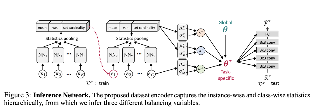
Focuses on extending MAML to unbalanced test datasets and out of distribution tasks. This is mostly implemented by adapting the inner gradient update according to the following formula:

where $*$ is abused in notation to “multiply if component in $\theta$ is a weight and add if component in $\theta$ is a bias” and $\circ$ represents element wise multiplication.

The components have the following roles:

• $\omega^\tau_c$ scales the gradient of all instances with class c. Allows to take larger gradient steps for classes with more examples in order to tackle class imbalance (Is this equivalent to computing a weighted loss?)
• $\gamma^\tau$ scales the size of gradient steps on a per task basis in order to tackle task imbalance. Reasoning: Larger tasks should have larger $\gamma$ because they can rely more on task-specific updates, while smaller tasks should have small $\gamma$ because they should rely more on meta-knowledge.
• $z^\tau$ relocates the initial weights for each task. This allows tasks which dissimilar (out of distribution) to the original meta-learnt tasks to be shifted further away in weight space, while task which are closes the meta-learnt tasks to remain closer. Tackles out-of-distribution tasks

The parameters are inferred using amortized variational inference, where the inference network is shared across all tasks and the parameters are computed conditionally on summary statistics derived from the task instances (see below).

In general, I find it very interesting how the authors incorporate additional terms into the inner gradient computation loop and how the inference of the associated parameters is implemented using variational inference on the summary statistics.

Meta Dropout: Learning to Perturb Latent Features for Generalization

Suggest to additionally learn how to perturb intermediate representation during meta learning using input dependent Dropout. This is done by computing parameters of the noise distribution dependent on the output of the previous layer. This results in the following preactivation:

The parameters of the function $ \mu $ and the weights of the layer $W$ are trained using the meta learning objects of MAML. Yet importantly, the weights of $\mu$ are not fitted in the inner training loop of MAML as this would allow the algorithm to “optimize away” the perturbation. Interestingly they use a lower bound to optimize the inner loop. This is not really motivated, but the authors draw a connection to variational inference, where q and p are from the same family and thus the KL would equal 0. The results look very good actually.

On Robustness of Neural Ordinary Differential Equations

Empirical study of Neural ODEs compared to ResNets. Show that they are more robust to random noise and to adversarial attacks. Further suggest Time-invariant steady state ODE (TisODE), to additionally improve robustness. This adds time invariance in the ODE function and a specific steady state condition.

They argue that the NeuralODE is more robust to perturbations as the ODE integral curves do not intersect (See Theorem 1). The argument is that due to the non intersecting property, each perturbation of less than $\epsilon$ would remain sandwiched within the $\epsilon$ ball and its distance from the unperturbed final position would remain upper bounded. Quite a cool insight. The extensions of the authors in TisODE aim at controlling the differences between neighboring integral curves to enhance NeuralODE robustness.

Why Not to Use Zero Imputation? Correcting Sparsity Bias in Training Neural Networks

Using Zero imputation induces a bias in the network! Often the prediction correlates with the fraction of imputed values more than with respect to the similarity of the instances! This effect is present across a large variety of datasets including medical data.

Authors coin term “Variable sparsity problem”, where the expected value of the output layer of a NN depends on the sparsity of the input data. The existence of this problem is derived theoretically based on a few assumptions.

Paper suggest that imputation with non zero values is helpful, by stabilizing the number of known entities. Phrase imputation as injecting plausible noise. Still it should be considered as injecting noise into the network!

Authors suggest to use sparsity normalization:

• Divide the input data by the L1 norm
• Then the average activation of the subsequent layer would be independent of data sparsity
• This is a simple preprocessing scheme of the input data!

Authors show theoretically that this preprocessing step can fix the variable sparsity problem. Empirical results are also in line with the theory.